Tutorial
Let’s start your survay of dielectric properties of various materials. The first thing you must do is to create a RiiDataFrame oject. The first trial will take a few minutes, because experimental data will be pulled down from Polyanskiy’s refractiveindex.info database and equi-spaced grid data will be obtained by interpolating the experimental data.
[1]:
import riip
ri = riip.RiiDataFrame()
Catalog file not found.
Cloning Repository...
Done.
Creating catalog file...
Done.
Creating raw data file...
Done.
Updating grid data file...
Done.
You can use some helper methods for your survay.
search
search(name: str) -> DataFrame
This method searches data that contain given name of material and return a catalog for them.
[2]:
ri.search("NaCl")
[2]:
| book | section | page | formula | tabulated | wl_min | wl_max | |
|---|---|---|---|---|---|---|---|
| id | |||||||
| 182 | NaCl | Li | 1 | f | 0.20 | 30.0000 | |
| 183 | NaCl | Querry | 0 | nk | 0.22 | 166.6667 |
[3]:
ri.search("sodium").head(5) # upper or lower case is not significant
[3]:
| book | section | page | formula | tabulated | wl_min | wl_max | |
|---|---|---|---|---|---|---|---|
| id | |||||||
| 127 | NaBr | Li | 1 | f | 0.210 | 34.0000 | |
| 182 | NaCl | Li | 1 | f | 0.200 | 30.0000 | |
| 183 | NaCl | Querry | 0 | nk | 0.220 | 166.6667 | |
| 229 | NaF | Li | 1 | f | 0.150 | 17.0000 | |
| 295 | NaI | Jellison | 1 | f | 0.436 | 0.6330 |
select
select(condition: str) -> DataFrame
This method make a query with the given condition and return a catalog. For example, if you want to find a material whose refractive index n is in a range 2.5 < n < 3 somewhere in the wavelength range 0.4μm < wl < 0.8μm:
[4]:
ri.select("2.5 < n < 3 and 0.4 < wl < 0.8").head(5)
[4]:
| book | section | page | formula | tabulated | wl_min | wl_max | |
|---|---|---|---|---|---|---|---|
| id | |||||||
| 23 | Al | Experimental data | Mathewson | 0 | nk | 0.495940 | 1.771200 |
| 118 | Bi | Experimental data | Hagemann | 0 | nk | 0.000002 | 6.199000 |
| 129 | TlBr | Palik | 1 | f | 0.570000 | 39.400000 | |
| 135 | C | Amorphous thin film | Larruquert | 0 | nk | 0.019656 | 10.079189 |
| 137 | C | Graphite | Djurisic-o | 0 | nk | 0.030996 | 10.332000 |
show
show(ids: int | Sequence[int]) -> DataFrame
This method shows the catalog for given ids.
[5]:
ri.show([23, 118])
[5]:
| book | section | page | formula | tabulated | wl_min | wl_max | |
|---|---|---|---|---|---|---|---|
| id | |||||||
| 23 | Al | Experimental data | Mathewson | 0 | nk | 0.495940 | 1.7712 |
| 118 | Bi | Experimental data | Hagemann | 0 | nk | 0.000002 | 6.1990 |
read
read(id, as_dict=False)
This method returns the contants of a page associated with the id.
[6]:
print(ri.read(23))
# this file is part of refractiveindex.info database
# refractiveindex.info database is in the public domain
# copyright and related rights waived via CC0 1.0

REFERENCES: "A. G. Mathewson and H. P. Myers. Absolute values of the optical constants of some pure metals, <a href=\"https://doi.org/10.1088/0031-8949/4/6/009\"><i>Phys. Scr.</i> <b>4</b>, 291-292 (1971)</a>"
COMMENTS: "298 K (24.85 °C)"
DATA:
  - type: tabulated nk
    data: |
        0.49594 0.77909 5.84012
        0.50606 0.81783 5.93033
        0.51660 0.85227 6.10134
        0.52759 0.89107 6.22848
        0.53906 0.94408 6.35541
        0.55104 1.00461 6.51991
        0.56356 1.06864 6.64394
        0.57667 1.14503 6.76839
        0.59040 1.21981 6.92733
        0.60480 1.30548 7.08550
        0.61992 1.40111 7.20855
        0.63582 1.50675 7.36684
        0.65255 1.62810 7.49338
        0.67018 1.77579 7.65855
        0.68880 1.94186 7.82757
        0.70848 2.13059 8.00246
        0.72932 2.33676 8.15233
        0.75142 2.57452 8.25398
        0.77490 2.87316 8.23135
        0.79990 3.03948 8.07703
        0.82656 2.93996 7.75521
        0.85506 2.52983 7.60921
        0.88560 2.13552 7.74987
        0.91840 1.81758 8.14270
        0.95372 1.57683 8.68829
        0.99187 1.41421 9.19239
        1.03320 1.31513 9.73291
        1.07812 1.24965 10.32287
        1.12713 1.22635 10.88595
        1.18080 1.22466 11.55421
        1.23984 1.25115 12.18874
        1.30510 1.29739 12.91059
        1.37760 1.34628 13.70447
        1.45864 1.42835 14.52722
        1.54980 1.50000 15.50000
        1.65312 1.58999 16.47811
        1.77120 1.75488 17.75048
SPECS:
    n_absolute: true
    wavelength_vacuum: true
    temperature: 298 K
references
references(id: int)
This method returns the REFERENCES of a page associated with the id.
[7]:
ri.references(23)
[7]:
plot
plot(id: int, comp: str = "n", fmt1: str = "-", fmt2: str = "--", **kwargs)
id: ID number
comp: ‘n’, ‘k’ or ‘eps’
fmt1 (Union[str, None]): Plot format for n and Re(eps), such as “-”, “–”, “:”, etc.
fmt2 (Union[str, None]): Plot format for k and Im(eps).
This plot uses 200 data points only. If you want more fine plots, use plot method of RiiMaterial explained below.
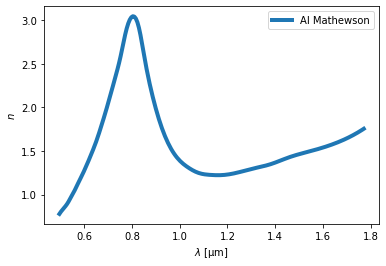
[8]:
ri.plot(23, "n")
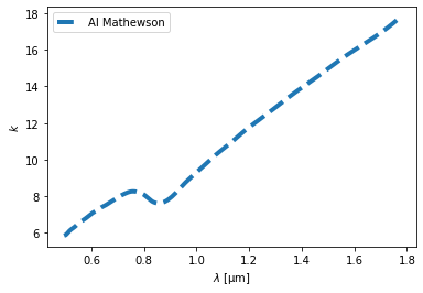
[9]:
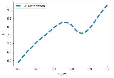
ri.plot(23, "k")
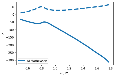
[10]:
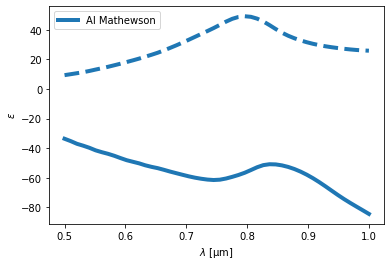
ri.plot(23, "eps")
material
material(params: dict) -> Material
This method returns Material-class instance for given parameter dict params.
params can includes the following parameters, * ‘id’: ID number. (int) * ‘book’: book value in catalog of RiiDataFrame. (str) * ‘page’: page value in catalog of RiiDataFrame. (str) * ‘RI’: Constant refractive index. (complex) * ‘e’: Constant permittivity. (complex) * ‘bound_check’: True if bound check should be done. Defaults to True. (bool) * ‘im_factor’: A magnification factor multiplied to the imaginary part of permittivity. Defaults to 1.0. (float)
[11]:
Al = ri.material({'id': 23})
type(Al)
[11]:
riip.material.Material
Using the created Material object, you can get refractive index n, extinction coefficient k, and dielectric function eps, and plot them. ### Material.n
n(wl: ArrayLike) -> ArrayLike
[12]:
Al.n(1.0) # refractive index at wavelength = 1.0μm
[12]:
1.3899282542977849
Material.k
k(wl: ArrayLikey) -> ArrayLike
[13]:
Al.k(1.0) # extinction coeficient at wavelength = 1.0μm
[13]:
9.29612443028388
Material.eps
eps(wl: ArrayLike) -> ArrayLike
[14]:
Al.eps(1.0) # permittivity at wavelength = 1.0μm
[14]:
(-84.48602887122551+25.84189200223893j)
Wavelengths wl can be a single complex value or an array of complex values.
[15]:
import numpy as np
wls = np.linspace(0.5, 1.6)
Al.eps(wls)
[15]:
array([ -33.67756077 +9.32237639j,  -37.37099091+10.76642941j,
        -40.48007076+12.53258237j,  -43.40382102+14.56069085j,
        -46.40772695+16.83596896j,  -49.24177749+19.32450842j,
        -51.87203854+22.05584598j,  -53.97258292+25.08305181j,
        -56.53596324+28.78875995j,  -58.88350388+32.86521087j,
        -60.71385987+37.1741283j ,  -61.57228729+41.55945809j,
        -60.12911702+46.32015037j,  -57.30534918+49.05004179j,
        -53.3025562 +47.83949057j,  -50.89837648+43.14679491j,
        -51.84632276+37.58238573j,  -54.80097964+33.65174018j,
        -59.37975454+30.91365925j,  -65.24676207+28.98346003j,
        -71.68601924+27.6368441j ,  -77.56359077+26.62565318j,
        -82.98698417+25.95615477j,  -88.58984464+25.65838341j,
        -94.49488142+25.59806765j, -100.57222728+25.6620527j ,
       -106.3896107 +25.86504049j, -111.80012917+26.22868897j,
       -117.37650002+26.73629885j, -123.56896814+27.35630896j,
       -129.97026563+28.05783746j, -135.99407702+28.81629758j,
       -141.62435872+29.63680412j, -147.25028441+30.54125595j,
       -153.19700042+31.53811566j, -159.4443053 +32.58896426j,
       -165.88659102+33.64199735j, -172.41898046+34.66687562j,
       -178.95505801+35.7002317j , -185.40696369+36.7933805j ,
       -191.7123965 +37.98898528j, -197.97226367+39.26611951j,
       -204.35066317+40.57994135j, -211.02107129+41.88287652j,
       -218.04602584+43.14590685j, -225.27973828+44.37584349j,
       -232.54532389+45.58404429j, -239.65527993+46.78308758j,
       -246.5066451 +47.9890921j , -253.186526  +49.22401988j])
Material.plot
plot(wls: np.ndarray, comp: str = "n", fmt1: str = "-", fmt2: str = "--", **kwargs)
wls: Wavelength [μm].
comp: ‘n’, ‘k’ or ‘eps’
fmt1 (Union[str, None]): Plot format for n and Re(eps), such as “-”, “–”, “:”, etc.
fmt2 (Union[str, None]): Plot format for k and Im(eps).
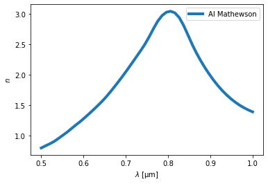
[16]:
import matplotlib.pyplot as plt
wls = np.linspace(0.5, 1.0)
Al.plot(wls, "n")
plt.show()
Al.plot(wls, "k")
plt.show()
Al.plot(wls, "eps")
plt.show()
[ ]: